Colorado River Resilience Investments Model (CRRIM)
This application contains the Colorado River Resilience Investments Model (CRRIM). CRRIM is an interactive tool that demonstrates the impacts of system-wide investments on both hydrologic and economic conditions within the Colorado River Basin. The overarching goal of CRRIM is to provide a tool that can be used to evaluate the relative cost-benefit characteristics of management actions that could be undertaken to reduce water supply risk and increase resiliency in the Colorado River Basin.
CRRIM was designed to operate as a back-end plug-in to the Colorado River Simulation System (CRSS) model, allowing users to undertake comparisons between two or more modeled CRSS scenarios in which the hydrologic results of particular management action(s) have been evaluated. It is also intended to allow the user to adjust economic assumptions and inputs in real-time in order to evaluate and/or optimize cost-benefits associated with paying for particular management actions among and between user groups. CRRIM is intended to function as a working model that can be readily adjusted based on feedback from stakeholders. Ultimately users can design CRSS input scenarios to simulate the impacts of particular management actions, have them processed through CRSS, and then add those scenarios to available menu of scenarios that can be compared in CRRIM to understand the potential hydrologic and economic results of particular management actions, and consider potential means of financing the implementation of those management actions.
In creating and making CRRIM widely available, we hope to spark a discussion about the potential feasibility, design, and approaches to financing management actions that could reduce water risk, including system conservation efforts.
How to Use, located in the menu on the left-hand side of this application, provides more information about use of this interactive tool. Scenario Descriptions provides a brief summary of the scenarios currently loaded into CRRIM. Under Inputs, users can modify four general categories of CRRIM model inputs to explore and/or optimize economic costs and benefits associated with potential management actions. Graphics include six categories of graphics displaying model outputs based on user defined inputs. About includes additional details on the analysis that supports this effort, including the CRRIM Framework, the current System Conservation Analysis and the Glossary.
DISCLAIMER
Definition of Terms
Administrative Cost: The amount of money that is assumed as the administrative cost of managing the cost of the user-defined program of management actions each year.
Annual Federal and State Funding: Money that is assumed to be contributed to the response fund each year by state and federal governments (or some other source). This can be used to supplement surcharge revenues, or to assess the annual cost of a program in the absence of surcharge revenues
Avoided Cost: The total cost (in U.S. dollars) that user groups are modeled to avoid incurring due to reductions in delivery shortages under the system conservation program scenario as compared to the baseline scenario.
Baseline Scenario: A comparison scenario output from CRSS that utilizes the same underlying hydrologic and demand assumptions as the active scenario, absent changes in supply or demand resulting from the management actions that are under evaluation in the active scenario.
Fund End of Year Balance: The amount of money (in U.S. dollars) remaining in the response fund at the end of each year after being credited by the amount of surcharges or debited by the cost of the management actions in that calendar year.
Implementation Cost: The amount of money (in U.S. dollars) that all user groups pay to the fund in the form of surcharges on water deliveries and/or surcharges on hydropower generation. This is calculated by multiplying deliveries by surcharges and/or hydropower generation by surcharges.
Insurance Return: The net balance of insurance premiums to insurance payouts as reflected in the scenario (i.e. net return or loss to the assumed insurance provider).
Insurance Payout: The amount of money paid by an assumed insurance provider to the response fund if the response fund balance drops below a specified level.
Insurance Premium: The amount of money paid to an assumed insurance provider each year in exchange for guaranteeing Insurance Payouts to the response fund.
Insurance Provider: To provide a means of assessing the potential cost/benefit of contingent financing for the management actions under consideration, the model allows the user to assume the existence of a source of funding that “insures” the response fund (guaranteeing the availability of funds in the event that revenues from the surcharge mechanism(s) are inadequate to cover the cost of management actions undertaken in the scenario. This function could be used to model the returns/losses of an actual insurer (who receives a premium each year in exchange for assuming the risk that the response fund is inadequate to cover the management costs in a scenario), or can be instead used to assess the degree to which proposed surcharge amounts are inadequate to cover program costs in a particular scenario.
Investment Return: The amount of money the fund gains each year as a result of investing the response fund balance according to user input assumptions.
Lake Elevations: A measure (in feet above sea level) of how much water is in the Lake Powell and Lake Mead reservoirs.
Rebates: The model allows the user to define a maximum response fund balance, above which surcharge revenues are either returned to the user groups or are not charged. Excess revenues are assumed to be returned to user groups in amounts proportional to their relative contribution. If the option to rebate investment returns is turned on, each user group’s portion of the total investment return will be rebated in addition to the surcharge revenues from that user group.
Response Expenditures: The amount of money paid out of the response fund to pay for the evaluated management actions (in the default scenarios, system conservation activities causing voluntary, temporary reductions in consumptive use). Response expenditures can be viewed both by state and by sector.
Response Fund: A pool of accumulated revenue from selected sources that is credited by the amount of revenue generated by surcharges or debited by the cost of the management actions undertaken in each year.
Savings: The modeled cost differences (in U.S. dollars) between the avoided cost and the implementation cost.
Surcharge: The user has the option to define a per acre-foot assessment for water used by particular user groups, and/or a charge assessed against hydropower users per GWh of hydropower generated. Surcharges can also be set to vary based on the relative amount of storage in Powell and Mead.
Surcharge Revenues: The amount of money each user group pays into the response fund as a function of surcharges on water delivered, or surcharges on hydropower generated. This is calculated by multiplying CRSS-modeled water deliveries and CRSS-modeled hydropower generation by the amounts of the user-defined surcharge(s).
Volume: The amount of water (in acre feet) saved by the proposed management actions (in the default scenarios, a basin-wide system conservation program involving voluntary & temporary compensated reductions in consumptive use).
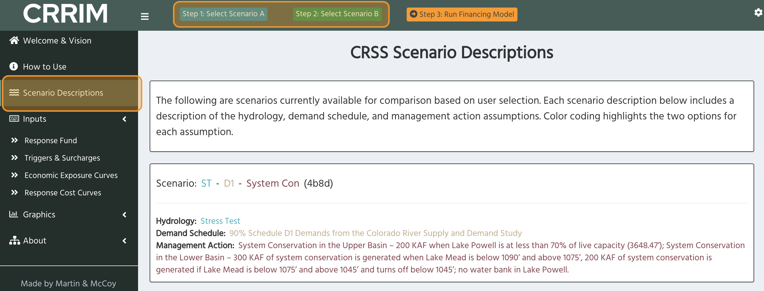
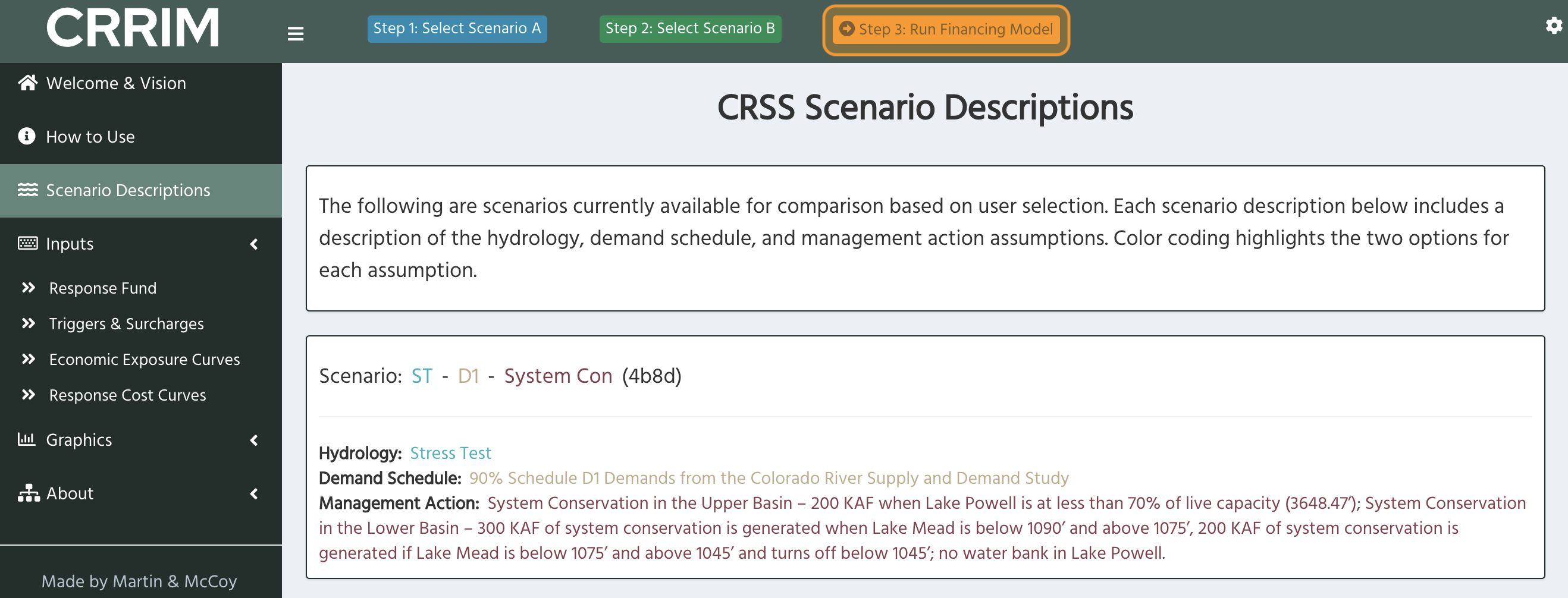
CRSS Scenario Descriptions
The following are scenarios currently available for comparison based on user selection. Each scenario description below includes a description of the hydrology, demand schedule, and management action assumptions. Color coding highlights the two options for each assumption.
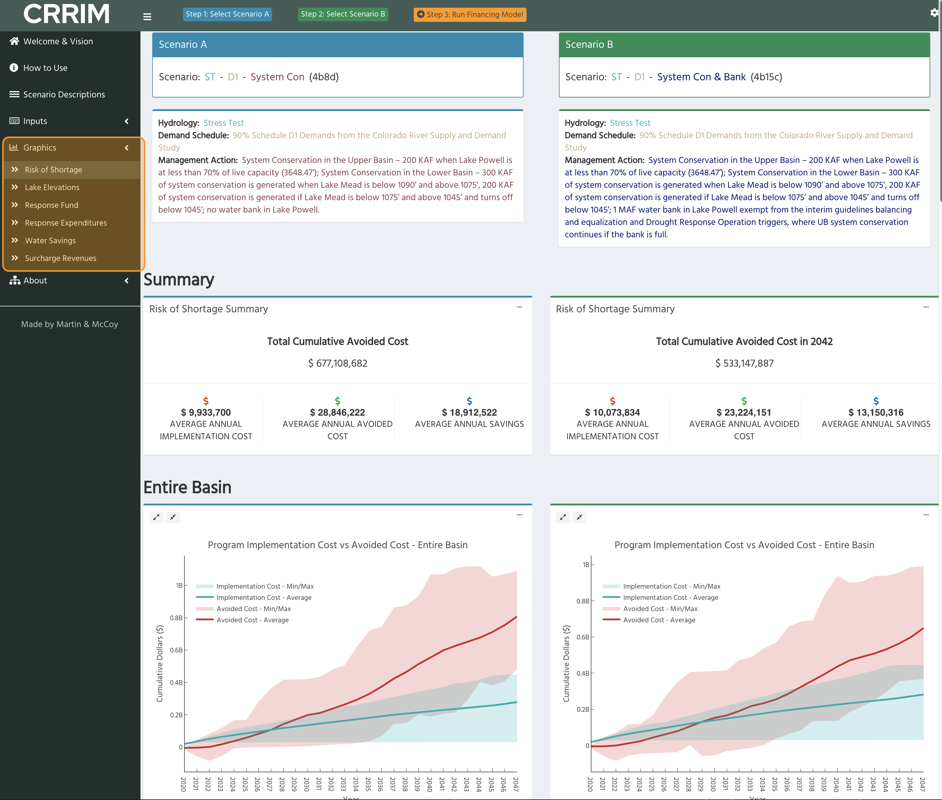
Scenario: ST - D1 - System Con (4b8d)
Hydrology: Stress Test
Demand Schedule: 90% Schedule D1 Demands from the Colorado River Supply and Demand Study
Management Action: System Conservation in the Upper Basin – 200 KAF when Lake Powell is at less than 70% of live capacity (3648.47’); System Conservation in the Lower Basin – 300 KAF of system conservation is generated when Lake Mead is below 1090’ and above 1075’, 200 KAF of system conservation is generated if Lake Mead is below 1075’ and above 1045’ and turns off below 1045’; no water bank in Lake Powell.
Scenario: ST - D1 - System Con & Bank (4b15c)
Hydrology: Stress Test
Demand Schedule: 90% Schedule D1 Demands from the Colorado River Supply and Demand Study
Management Action: System Conservation in the Upper Basin – 200 KAF when Lake Powell is at less than 70% of live capacity (3648.47’); System Conservation in the Lower Basin – 300 KAF of system conservation is generated when Lake Mead is below 1090’ and above 1075’, 200 KAF of system conservation is generated if Lake Mead is below 1075’ and above 1045’ and turns off below 1045’; 1 MAF water bank in Lake Powell exempt from the interim guidelines balancing and equalization and Drought Response Operation triggers, where UB system conservation continues if the bank is full.
Scenario: ST - A - System Con (17b18d)
Hydrology: Stress Test
Demand Schedule: Schedule A Demands from the Colorado River Supply and Demand Study
Management Action: System Conservation in the Upper Basin – 200 KAF when Lake Powell is at less than 70% of live capacity (3648.47’); System Conservation in the Lower Basin – 300 KAF of system conservation is generated when Lake Mead is below 1090’ and above 1075’, 200 KAF of system conservation is generated if Lake Mead is below 1075’ and above 1045’ and turns off below 1045’; no water bank in Lake Powell.
Scenario: ST - A - System Con & Bank (17b19c)
Hydrology: Stress Test
Demand Schedule: Schedule A Demands from the Colorado River Supply and Demand Study
Management Action: System Conservation in the Upper Basin – 200 KAF when Lake Powell is at less than 70% of live capacity (3648.47’); System Conservation in the Lower Basin – 300 KAF of system conservation is generated when Lake Mead is below 1090’ and above 1075’, 200 KAF of system conservation is generated if Lake Mead is below 1075’ and above 1045’ and turns off below 1045’; 1 MAF water bank in Lake Powell exempt from the interim guidelines balancing and equalization and Drought Response Operation triggers, where UB system conservation continues if the bank is full.
Scenario: CC - D1 - System Con (9b10d)
Hydrology: Downscaled climate change using CMIP-3
Demand Schedule: 90% Schedule D1 Demands from the Colorado River Supply and Demand Study
Management Action: System Conservation in the Upper Basin – 200 KAF when Lake Powell is at less than 70% of live capacity (3648.47’); System Conservation in the Lower Basin – 300 KAF of system conservation is generated when Lake Mead is below 1090’ and above 1075’, 200 KAF of system conservation is generated if Lake Mead is below 1075’ and above 1045’ and turns off below 1045’; no water bank in Lake Powell.
Scenario: CC - D1 - System Con & Bank (9b14c)
Hydrology: Downscaled climate change using CMIP-3
Demand Schedule: 90% Schedule D1 Demands from the Colorado River Supply and Demand Study
Management Action: System Conservation in the Upper Basin – 200 KAF when Lake Powell is at less than 70% of live capacity (3648.47’); System Conservation in the Lower Basin – 300 KAF of system conservation is generated when Lake Mead is below 1090’ and above 1075’, 200 KAF of system conservation is generated if Lake Mead is below 1075’ and above 1045’ and turns off below 1045’; 1 MAF water bank in Lake Powell exempt from the interim guidelines balancing and equalization and Drought Response Operation triggers, where UB system conservation continues if the bank is full.
Scenario: CC - A - System Con (11b12d)
Hydrology: Downscaled climate change using CMIP-3
Demand Schedule: Schedule A Demands from the Colorado River Supply and Demand Study
Management Action: System Conservation in the Upper Basin – 200 KAF when Lake Powell is at less than 70% of live capacity (3648.47’); System Conservation in the Lower Basin – 300 KAF of system conservation is generated when Lake Mead is below 1090’ and above 1075’, 200 KAF of system conservation is generated if Lake Mead is below 1075’ and above 1045’ and turns off below 1045’; no water bank in Lake Powell.
Scenario: CC - A - System Con & Bank (11b16c)
Hydrology: Downscaled climate change using CMIP-3
Demand Schedule: Schedule A Demands from the Colorado River Supply and Demand Study
Management Action: System Conservation in the Upper Basin – 200 KAF when Lake Powell is at less than 70% of live capacity (3648.47’); System Conservation in the Lower Basin – 300 KAF of system conservation is generated when Lake Mead is below 1090’ and above 1075’, 200 KAF of system conservation is generated if Lake Mead is below 1075’ and above 1045’ and turns off below 1045’; 1 MAF water bank in Lake Powell exempt from the interim guidelines balancing and equalization and Drought Response Operation triggers, where UB system conservation continues if the bank is full.
CRRIM Framework
The Colorado River Resilience Investments Model (CRRIM) consists of a three-part analytical framework (1) CRSS Scenarios, (2) Economic Exposures Analysis, and (3) Financing Mechanism:
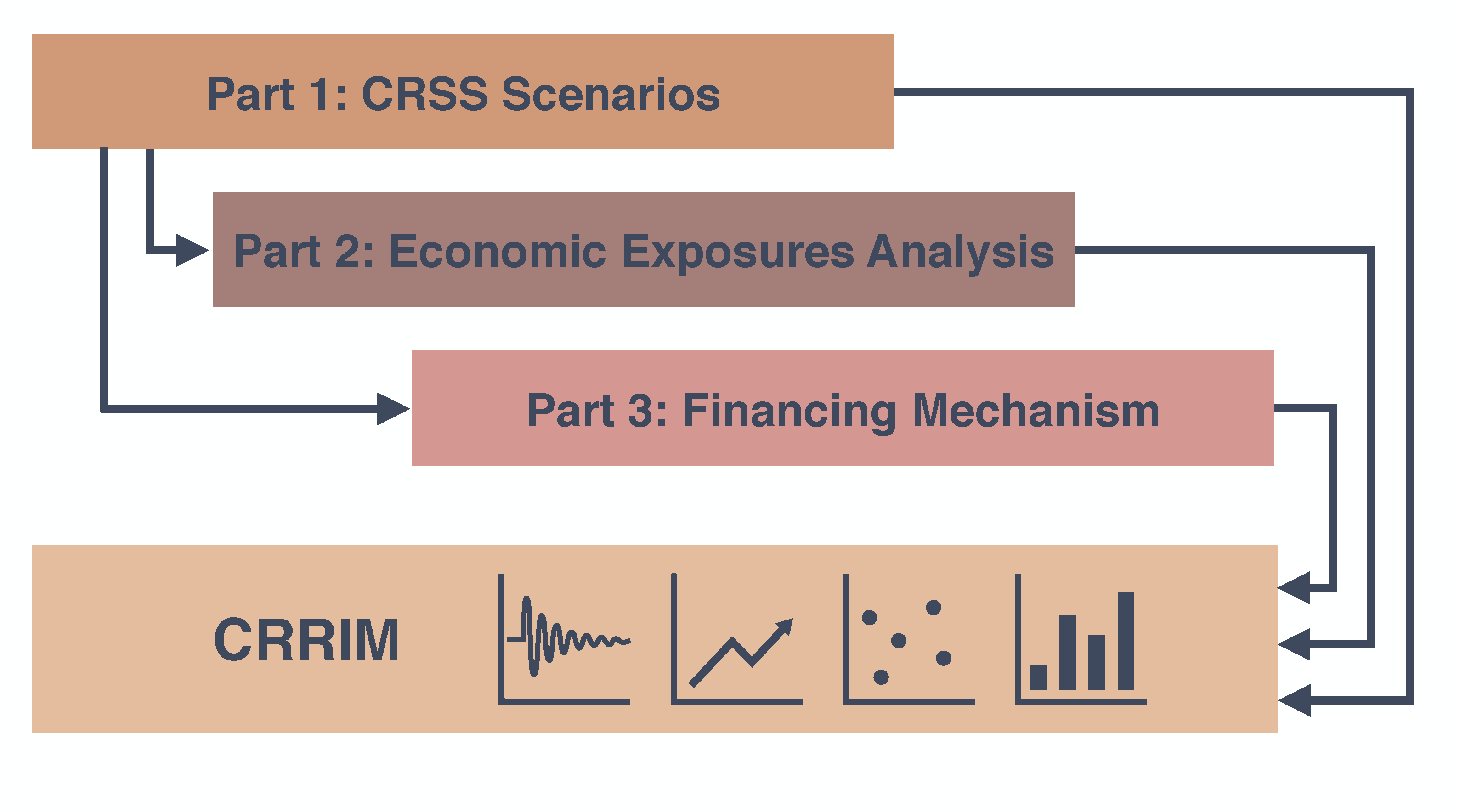
Part 1: CRSS Scenarios
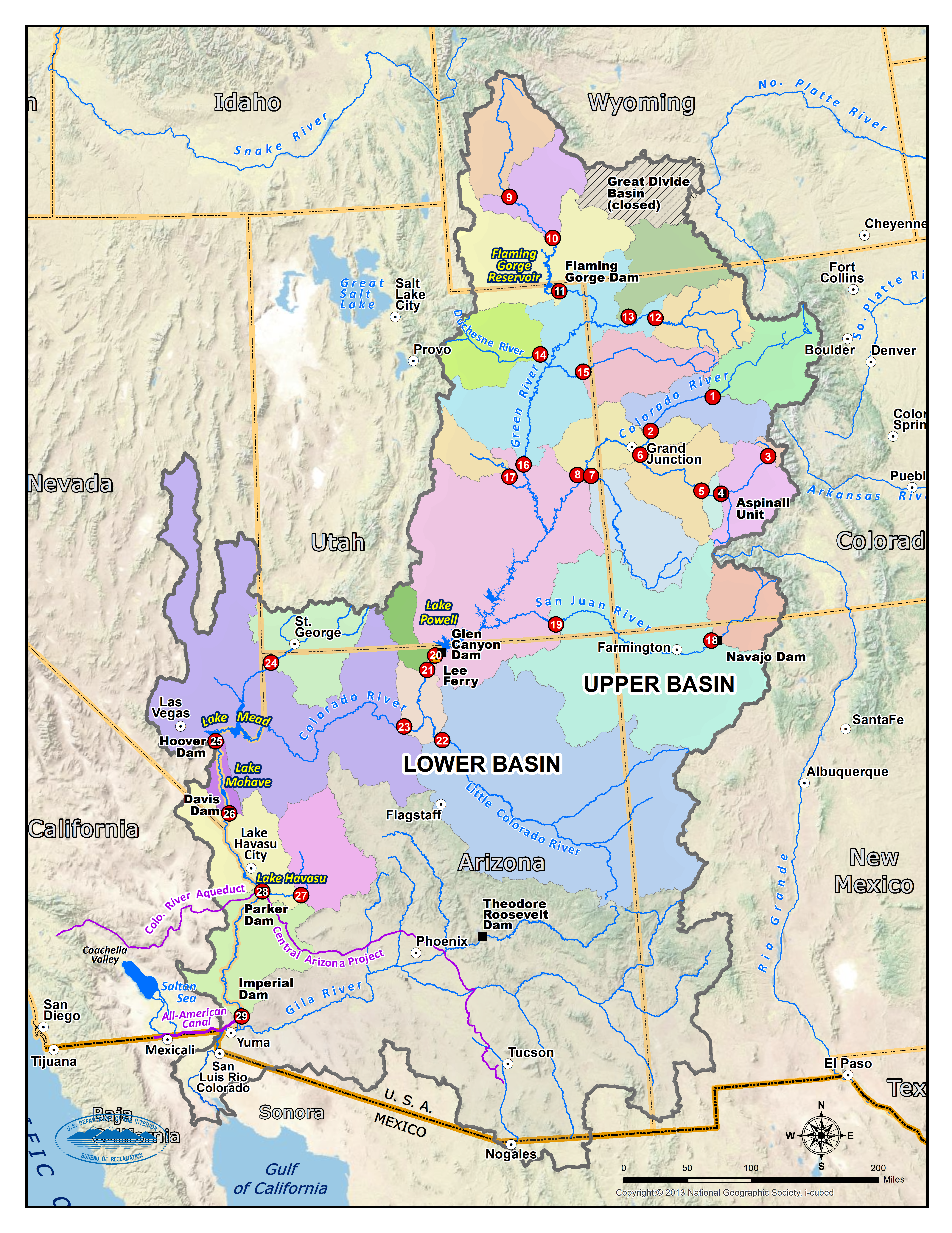
CRRIM evaluates and displays the results of various combinations of water supply, demand and management scenarios (e.g. implementation of Lower Basin Drought Contingency Plan, Upper Basin Drought Response Operations, system conservation programs, and Minute 323) that have been run through the Colorado River Simulation System (CRSS) model. CRSS is a comprehensive model of the Colorado River system implemented in the commercial river modeling software known as RiverWare. CRSS is used by the U.S. Bureau of Reclamation to forecast reservoir operations and to make long-term planning decisions on the Colorado River.
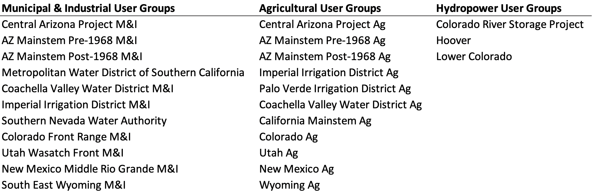
To provide the scenario inputs for CRRIM, raw CRSS outputs are processed to obtain water user shortage, water user deliveries, hydropower generation, and reservoir elevation data. Water users are broken down into municipal and industrial user groups, agricultural user groups and hydropower user groups (Table 1). These user groups are preliminary groupings, and are based on the expectation that replacement supply costs would be approximately similar within each user group. The groupings are extremely flexible and can be made more granular or coarse in future iterations of CRRIM.
For additional methods on the conversion of CRSS outputs to user groups see CRSS Methods.
Table 1: User Groups
Part 2: Economic Exposure Analysis
The economic exposure analysis calculates the economic impacts of reductions in water deliveries to water users and to hydropower production as a result of (1) policy shortages generated by the 2007 Interim Guideline and Drought Contingency Plan contributions; and (2) hydrologic shortages caused when water adequate to meet demands either can no longer be delivered through the infrastructure in the Lower Basin and/or when water is physically unavailable due to spatial variability of low flows in the Upper Basin.
CRRIM estimates the economic exposure for particular water user groups by assuming a cost of replacement water for that user group sufficient to offset any policy shortage and/or hydrologic shortage predicted by the model. The analysis thus assumes that the Colorado River supply will be replaced with other surface water supplies, groundwater supplies, recycled water, and/or water conservation to eliminate the gap between water demand and supplies; however, the cost curve could also be used to define a marginal economic cost associated with actual shortage.
Available replacement supplies and costs were estimated from water management options included in the 2012 Colorado River Water Supply and Demand Study and subsequent 2015 Moving Forward Effort. In some planning areas (e.g. Coastal Southern California), regional water management economic studies were reviewed to include more refined unit replacement supply costs. The cost curves used in this analysis can be modified by the user.
Economic exposure for hydropower is calculated by determining the total hydropower generation predicted by the CRSS model run, the difference between modeled generation and the contract allocations, and multiplying any deficits in production by energy spot market prices. Please see the Hydropower Economic Exposure Methods for additional detail.
Finally, CRRIM calculates the economic benefits or avoided costs associated with the management actions under consideration by comparing the economic exposure of the scenario of interest to the economic exposure of a baseline scenario. This comparison is used to assess the overall economic benefit or avoid cost of the modeled intervention for each water user group.
Part 3: Financing Mechanism
The CRRIM finance mechanism is based on a monthly balance sheet that calculates a net Reponse Fund balance based on the revenues generated by surcharges and/or appropriations in a particular year, the cost of the modeled reductions in water use/increases in supply, other program costs (e.g. insurance premiums), insurance payouts, investment returns, and any rebate program. The financing mechanism is designed to evaluate the revenue/cost relationship over a 25-42 year time period of the modeled scenario. The mechanism allows the user to define and modify any of the following revenue streams:
1: Hydropower surcharges based on elevation triggers in Lake Powel and Lake Mead, as a charge for every GWH of energy produced;
2: Municipal surcharges based on elevation triggers in Lake Mead and Lake Powell, as a charge for every acre-foot of water delivered to the user group;
3: Annual federal fuding (all sources);
4: Annual state funding (all sources);
5: Returns from the investment of the funding sources above;
6: Insurance payouts if the projected expenditures of the fund exceed the fund balance.
System Conservation Analysis
The default scenarios utilized in CRRIM are focused on assessing the viability of a basin-wide system conservation program (to reduce water supply and economic risks driven by continued drought, high temperatures, and reduced water availability in the Colorado River Basin). System conservation refers to voluntary, temporary reductions in consumptive use. Generally, Upper Basin stakeholders tend to refer to this as “demand management,” while Lower Basin stakeholders typically use the term “system conservation” to discuss the same concept. Given that the program investigated here is basin-wide, the overarching term “system conservation” was chosen for simplicity.
Drawing on current risk modeling, demand and climate change projections, and experience with the System Conservation Pilot Program over the last few years, CRRIM has been used to analyze whether a basin-wide system conservation program could reduce consumption (or export) of Colorado River water, decrease risk to water users, and provide an important source of alternative revenue for agricultural communities. Two hypotheses guided this analysis.
System Conservation Program Hypotheses
A: Adequate revenue can be generated to cover the costs of the system conservation program through a strategic combination of:
- Hydropower surcharges,
- Municipal surcharges,
- Federal & state appropriations and reallocation of existing sources,
- Investment returns; and
- An emergency insurance program.
B: A system conservation program designed to intervene early and often, with or without a water bank in the Colorado River Storage Project (CRSP) units, would reduce risk to water users and incentivize investment in a long-term financing mechanism to pay for annual system conservation, and could create benefits sufficient to offset the costs of surcharges and/or appropriations.
System Conservation Program Design
The system conservation scenarios created were designed to intervene early and often to prevent critically low elevations in both Lake Powell and Lake Mead
In the Upper Basin, 200 KAF of system conservation is generated annually when Lake Powell was at less than 70% of live capacity (3648.47’) and remained in place unless Lake Powell exceeded 70% of live capacity.
In the Lower Basin, 300 KAF of system conservation is generated when Lake Mead is below 1090’ and above 1075’, 200 KAF of system conservation is generated if Lake Mead is below 1075’ and above 1045’ and turns off below 1045’. The Lower Basin system conservation was designed to layer on top of early Drought Contingency Plan contributions, but ramp down as Drought Contingency Plan contributions increase (essentially allowing required DCP contributions to replace initial system conservation efforts).
The Upper Basin water bank scenario modeled a 1 MAF bank in Lake Powell that was exempt from the interim guidelines balancing and equalization, and which was also exempt from Drought Response Operation triggers. If the bank reaches maximum storage capacity, system conservation does not stop; once the bank is full, excess system conservation is treated as system water in the CRSP Units.
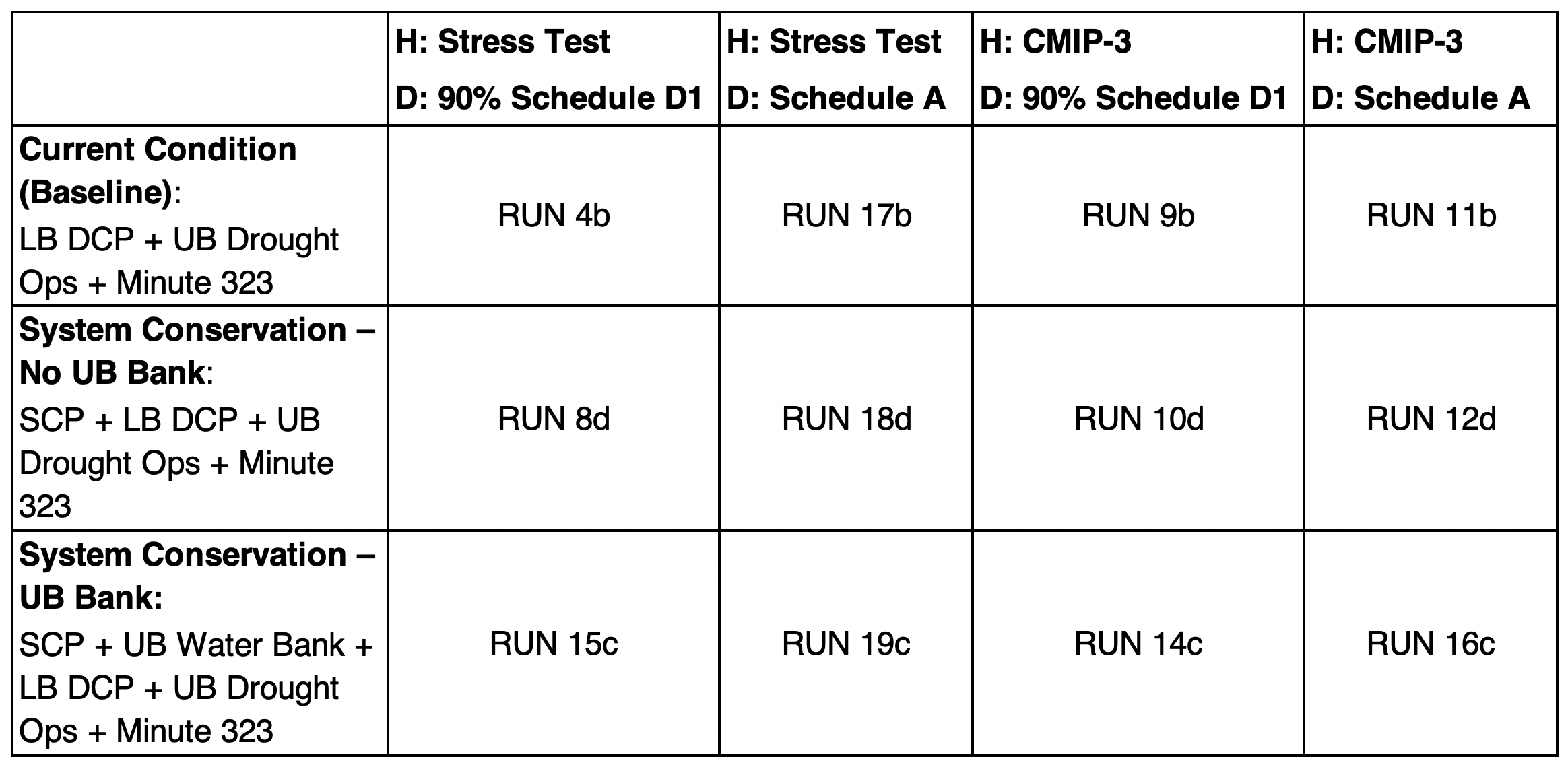
The system conservation scenarios were combined with two demand schedules, 90% of D1 Demand Scenario and Demand Scenario A, from the 2012 Colorado River Basin Water Supply and Demand Study, and two hydrology scenarios, Stress Test from Colorado River System Projected Future Conditions - Alternative Future Hydrology Scenarios and CMIP-3 from 2012 Colorado River Basin Water Supply and Demand Study.
This resulted in twelve (12) CRSS scenarios (Table 1). These twelve scenarios have been used to analyze the system conservation program hypotheses. Please see CRSS Assumptions for additional modeling details.
Table 1. CRSS Scenarios
How to Use
The Colorado River Resilience Investments Model (CRRIM) is designed to optimize user input. To learn how to use CRRIM, watch the informational how-to video (under construction) or follow the instructions below.
Step 1: Select Inputs
On the menu on the left-hand side of the application, click “Inputs.” Four input categories are shown: Response Fund, Triggers & Surcharges, Economic Exposure Curves, and Response Cost Curves. Click each input category and choose the desired inputs for evaluation in the model run.
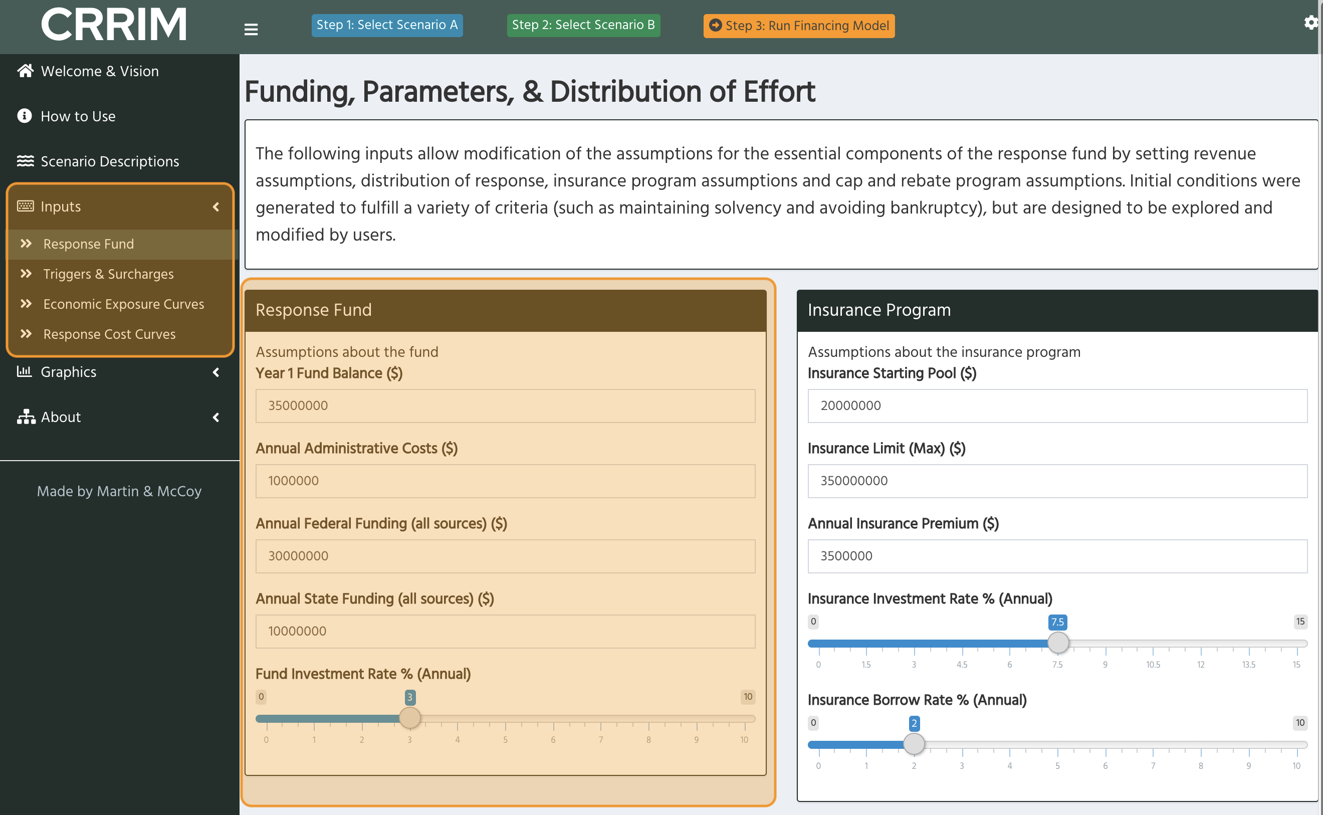
1: Response Fund: Input assumptions about the Response Fund, insurance program, and distribution of demand reduction or supply enhancement effort between the seven U.S. Colorado River Basin states, and the nature of the Response Fund cap and rebate program.
2: Triggers & Surcharges: Choose trigger elevations and municipal and/or hydropower surcharge amounts ($) for up to four different elevations in Lake Powell and Lake Mead. Customize surcharges by user group.
3: Economic Exposure Curves: For each user group input exposure data and create cost curves including (1) the volume in acre-feet, and (2) the cost in acre-feet. Click “Save” below the VolumeAF and CostAF table after entering the information. The graphic below the table will update after the information is saved. Once all cost curves have been updated, click 'Recalculate economic exposure model' at the top of the page.
4: Response Cost Curves: For each state (Arizona, California, Nevada, Colorado, Utah, New Mexico, and Wyoming) and each sector (agricultural, municipal, and tribal) choose (1) the percent of water savings to be generated, (2) the volume in acre-feet, and (3) the cost in acre-feet. Click “Save” below the VolumeAF and CostAF table after entering the information. The graphic below the table will update after the information is saved.
Note: re-calculating economic exposure may take up to 9 minutes due to the significant size of the underlying data
Step 2: Select Scenario A and Scenario B
On the menu on the left-hand side of the application, click Scenario Descriptions and review the scenario options. On the top bar of the application, click “Select Scenario A” and choose one of the scenario options from the drop down. Next, on the top bar of the application, click “Select Scenario B” and choose one of the scenario options from the drop down.
Step 3: Click Run Financing Model
To run the results, click “Run Financing Model” in the top bar of the application.
NOTE: This may take up to 8 minutes, particularly for any of the Climate Change (CMIP-3) scenarios due to the significant size of the underlying data.
Step 4: Review Graphics
On the menu on the left-hand side of the application, click “Graphics”. Next, select from six categories of graphics—Risk of Shortage, Lake Elevations, Response Fund Health, Response Expenditures, Water Savings, and Surcharge Revenues.
Each category displays a series of graphs that illustrate the effectiveness of the chosen inputs and scenarios and can be used to inform potential modifications of inputs as well as understand benefits and risk reduction potential.
Step 5: Repeat
Repeat steps 1-3 to generate other financing model results
Under the Hood
The Colorado River Resilience Investments Model (CRRIM) draws on data from CRSS and the economic exposure analysis and financing mechanism to generate graphical illustrations. Each part of the model involves discrete steps outlined below.
STEP 1: Load input data
STEP 2: Set changeable inputs
STEP 3: Calculate benefits
STEP 4: Calculate intervention (Phase 1: system conservation program)
STEP 5: Create water cost curves and calculate expenditures
STEP 6: Calculate revenue
STEP 7: Compute balance sheets (monthly remaining balance, rebates, monthly insurance payouts, monthly insurance balance, monthly investment gains, end of month balance, and monthly starting balance))
STEP 8: Conversions: cumulative and annual
The graphic below outlines inputs, intermediate steps and outputs of CRRIM.
CRSS Scenarios
Upper and lower Basin system conservation volumes and associated trigger elevations
Economic Exposure Analysis
The economic exposure analysis calculates the economic impact of reductions in water deliveries to water users as a result of shortages (e.g. IG shortages, LB DCP), as well as impacts to hydropower production.
Overview
Economic exposure for water users is calculated based on the average cost of replacement water for each of the user groups. These cost curves are currently static but can be shared and modified upon request.
Economic exposure for hydropower is calculated by determining the total hydropower generation, the difference between generation and the contract allocations and multiplying any deficits in production by energy spot market prices.
The economic benefits of the investment are calculated by comparing the economic exposure of the scenario of interest to the economic exposure of a baseline scenario. This results in the overall economic benefit of the intervention for each water user group.
The results of the economic exposure analysis are found in the 'Risk of Shortage' graphics page.
Funding, Parameters, & Distribution of Effort
The following inputs allow modification of the assumptions for the essential components of the response fund by setting revenue assumptions, distribution of response, insurance program assumptions and cap and rebate program assumptions. Initial conditions were generated to fulfill a variety of criteria (such as maintaining solvency and avoiding bankruptcy), but are designed to be explored and modified by users.
Response Fund
Insurance Program
State Effort
Upper Basin (must add to 100%)
Lower Basin (must add to 100%)
Cap & Rebate Program
Triggers & Surcharges
The following allows modification of the triggers associated with surcharge revenues for municipal and hydropower user groups. Initial conditions were generated to fulfill a variety of criteria (such as maintaining solvency and avoiding bankruptcy), but are designed to be explored and modified by users. To turn off the surcharge program, set all user group values to zero.
Upper Basin Summary Table (User Selected)
Lower Basin Summary Table (User Selected)
Response Cost Curves
The following allows modification of the response curves to calculate cost of the management action or response. Distribution of response by state can be set in Response Fund. Sectoral distribution of response is set by state in the following tables. Additionally response curves cost per quantity of response can be modified for each sector by state. Make sure to save any changes in each response curve to ensure the model integrates any changes.
Arizona
Agricultural
Edit % & Table, then click Save
Municipal
Edit % & Table, then click Save
Tribal
Edit % & Table, then click Save
California
Agricultural
Edit % & Table, then click Save
Municipal
Edit % & Table, then click Save
Tribal
Edit % & Table, then click Save
Nevada
Agricultural
Edit % & Table, then click Save
Municipal
Edit % & Table, then click Save
Tribal
Edit % & Table, then click Save
Colorado
Agricultural
Edit % & Table, then click Save
Municipal
Edit % & Table, then click Save
Tribal
Edit % & Table, then click Save
Utah
Agricultural
Edit % & Table, then click Save
Municipal
Edit % & Table, then click Save
Tribal
Edit % & Table, then click Save
New Mexico
Agricultural
Edit % & Table, then click Save
Municipal
Edit % & Table, then click Save
Tribal
Edit % & Table, then click Save
Wyoming
Agricultural
Edit % & Table, then click Save
Municipal
Edit % & Table, then click Save
Tribal
Edit % & Table, then click Save
Economic Exposure Curves
The following allows modification of the economic exposure curves to calculate the economic impacts of reductions in water deliveries to water users. The economic exposure curves were developed by averaging costs of replacement water for each user group sufficient to offset any shortage. Default economic exposure curves can be adjusted to more accurately reflect the replacement supply costs associated with each water user group. Make sure to save any changes in each economic exposure curve to ensure the model integrates any changes. Once all modifications are made, click Recalculate Economic Exposure Model.
Agriculture
Colorado Agriculture
Edit table, then click Save
New Mexico Agriculture
Edit Table, then click Save
Utah Agriculture
Edit Table, then click Save
Wyoming Agriculture
Edit Table, then click Save
Arizona Main Pre-1968 Agriculture
Edit Table, then click Save
Arizona Main Post-1968 Agriculture
Edit Table, then click Save
Imperial Irrigation District Agriculture
Edit Table, then click Save
Palo Verde Irrigation District Agriculture
Edit Table, then click Save
Coachella Valley Water District Agriculture
Edit Table, then click Save
California Mainstem Agriculture
Edit Table, then click Save
CAP Agriculture
Edit Table, then click Save
Municipal & Industrial
Southern Nevada Water Authority
Edit Table, then click Save
New Mexico Middle Rio Grande
Edit Table, then click Save
Utah Wasatch Front
Edit Table, then click Save
Southeastern Wyoming
Edit Table, then click Save
Colorado Front Range
Edit Table, then click Save
Metropolitan Water District of Southern California
Edit Table, then click Save
Imperial Valley Irrigation District MI
Edit Table, then click Save
Coachella Valley Water District MI
Edit Table, then click Save
AZ Mainstem Pre-1968 MI
Edit Table, then click Save
AZ Mainstem Post-1968 MI
Edit Table, then click Save
Central Arizona Project MI
Edit Table, then click Save
Hydrologic Shortage
Upper Basin Hydrologic Shortage
Edit Table, then click Save
Lower Basin Hydrologic Shortage
Edit Table, then click Save
Scenario A
Scenario B
Summary
Risk of Shortage Summary
Total Cumulative Avoided Cost
Risk of Shortage Summary
Total Cumulative Avoided Cost in 2042
Entire Basin
Upper Basin
Lower Basin
Upper Basin Municipal
Lower Basin Municipal
Upper Basin Hydropower
Lower Basin Hydropower
Scenario A
Scenario B
Lake Mead Elevation
Lake Powell Elevation
Scenario A
Scenario B
Summary
Annual Federal Funding (all sources)
Annual State Funding (all sources)
Fund Health Summary
Fund Health Summary
Fund Balance
Insurance Program
Revenues vs. Expenditures
Revenues vs. Expenditures (Difference)
Surcharge Revenues After Rebates
Scenario A
Scenario B
Expenditures by Basin
Expenditures by State
Expenditures by Water Sector
Average Annual Expenditures by Water Sector
Average Annual Expenditures by Water Sector
Expenditures by State - Map
Scenario A
Scenario B
Volume by Basin
Volume by State
Average Annual Response Volume by Water Sector
Average Annual Volume by Water Sector (Acre Feet)
Volume by Water Sector
Volume by State - Map
Scenario A
Scenario B
Surcharge Revenues by Basin
Surcharge Revenues by User Group
Average Annual Surcharge Revenue